Guest. Introduction to Reinforcement Learning

Given by: Asst. Prof. Gokhan Alcan

Recap

1. Define cost-to-go $V_k(x)$ (min cost from time k to N)
2. Split the problem ( Current step + Future)
3. The Result (Recursive Optimality)

Pro:

1. Decoupling: dont solve the full trajectory at once, solve one step at a time, working backwards from N to 0.
2. The RL connection:
   • in optimal control, we calculate V using the model f.
   • in RL, we learn Q directly so we can pick u without needing f.

From OC to RL

最优控制 (Optimal Control)	强化学习 (Reinforcement Learning)
状态 (State) $x_k$	状态 (State) $s_t$
控制输入 (Control Input) $u_k$	动作 (Action) $a_t$
阶段代价 (Stage Cost) $\ell(x, u)$	回报 (Reward) $r(s, a) \approx -\ell$
终端代价 (Terminal Cost) $\ell_N(x)$	终端回报 (Terminal Reward)
动力学 (Dynamics) $f(x, u)$	环境 (Env.) $P(s' \mid s, a)$
时界 (Horizon) $N$	折扣因子 (Discount) $\gamma$
控制器 (Controller)	策略 (Policy) $\pi(a \mid s)$

graph LR
    Agent --->|Action a_t| Environment
    Environment --->|State s_t+1 <br> Reward r_t| Agent

RL Objective

Maximize the expected cumulative discounted reward:

$$J(\pi) = \mathbb{E}_{\tau \sim \pi} \left[ \sum_{t=0}^{\infty} \gamma^t r(s_t, a_t) \right]$$

• $\gamma \in [0, 1)$：折扣因子 (Discount factor)，在无限时界问题中替代了有限时界 $N$。
• $\mathbb{E}$：期望值 (Expectation)，用于处理环境或策略中的随机性 (stochasticity)。

The Vocabulary of RL

核心概念 (Concept)	数学符号 (Notation)	倒立摆示例 (Cart-Pole Example)
策略 (Policy) (The Controller)	$\pi_{\theta}(a \mid s)$ (随机性策略 Stochastic) $\mu_{\theta}(s)$ (确定性策略 Deterministic)	“如果杆子向右倾斜 ($s$)，以 0.9 的概率向右推 ($a$)。”
价值函数 (Value Functions) (The Critic)	$V^{\pi}(s) = \mathbb{E}\left[\sum \gamma^t r_t\right]$ $Q^{\pi}(s, a)$	$V^{\pi}$：“当前这个状态有多好？” $Q^{\pi}$：“现在立刻向左推有多好？”
优势函数 (Advantage) (Relative Value)	$A^{\pi}(s, a) = Q^{\pi}(s, a) - V^{\pi}(s)$	“相比于当前策略的平均表现，做这个动作能好多少？”
轨迹 (Trajectory) (Rollout)	$\tau = (s_0, a_0, r_0, s_1, \dots)$	从开始（杆子竖直）到失败（杆子倒下）的单次完整模拟运行。

Critical Assumptions

1. Environment Assumptions (The Physics)
   • Markov Property: the state $s_t$ is sufficient. History doesnt matter (ONLY the current state matter, its enough to transit to next state)
   • Stationarity: The environment dynamics $P(s'|s,a)$ do not change over time. (mass or something stays constant)
   • Ergodicity & Coverage: The agent can reach all relevant states with non-zero probability. (Implication: If we stop exploring (greedy), we violate this and stop learning)
2. Structural Assumptions
   • Reward Boundedness: Rewards are finite. We use a discount factor $\gamma < 1$ to ensure the infinite sum converges:
   $$\sum_{t=0}^{\infty} \gamma^t r_t < \infty$$
   • Function Approximation Class：
     • Linear: Convex optimization, convergence guarantees, able to find global optima.
     • Neural Networks: Non-convex, no strong guarantees, but scales to high dimensions (images, complex dynamics)
   • Deep Q-Networks
     • $Q_{\theta}(s,a)$: Parameterized by weights $\theta$.
     • $Q_{\phi}(s,a)$: Parameterized by weight $\phi$ (a frozen copy of $\theta$).

Bell man optimality for RL

1. recursive optimality(OC)

$$V_k(x) = \min_{u} \Big[ \ell(x, u) + V_{k+1}(f(x, u)) \Big]$$

2. Action value $Q_k$ current state cost + remaining states’ within the bracket as the action value, consequently, the state value function can be simplified to minimising $Q_k$:

$$Q_k(x, u) := \ell(x, u) + V_{k+1}(f(x, u))$$ $$V_k(x) = \min_{u} Q_k(x, u)$$

3. subsitute $V_{k+1} = \min_{u'} Q_{k+1}$ into Q. Recursive form, purely in $Q$

$$Q_k(x, u) = \ell(x, u) + \min_{u'} Q_{k+1}\big(f(x, u), u'\big)$$

4. Bellman optimality equation in RL

$$Q^*(s, a) = r(s, a) + \gamma \max_{a'} Q^*(s', a')$$

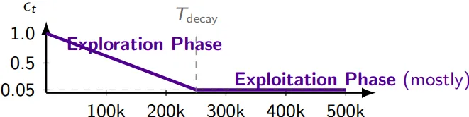
Exploration policy: $\epsilon$ - greedy schedule. Experience Replay: Buffer D of past transitions $\implies$ decorrelate samples. TD target & loss:: 在训练时，我们通过当前步的奖励 $r$ 和下一步的极大动作价值来构建 TD 目标值 (TD Target) $y$：

$$y = r + \gamma \max_{a'} Q_{\phi}(s', a')$$

随后，利用均方误差 (MSE) 构建 损失函数 (Loss Function)，通过梯度下降来更新当前网络参数 $\theta$：

$$\mathcal{L}(\theta) = \big( Q_{\theta}(s, a) - y \big)^2$$

---

Target update rule

为了解决训练中的非平稳目标问题，DQN 引入了目标网络 (Target Network)：

• $Q_{\theta}$：当前网络 (Online Network)，其参数 $\theta$ 在每一步都在通过梯度下降进行实时更新。
• $Q_{\phi}$：目标网络 (Target Network)，其参数 $\phi$ 保持冻结，仅进行周期性同步 (Periodic copy)：

$$\phi \leftarrow \theta \quad (\text{every } C \text{ steps})$$

Explorations schedule The exploration rate $\epsilon_t$ linearly decays from an initial value to a minimum floor over a fixed duration $T_{decay}$, then remains constant.

$$\epsilon_t = \max \left( \epsilon_{\text{end}}, \, \epsilon_{\text{start}} - \frac{\epsilon_{\text{start}} - \epsilon_{\text{end}}}{T_{\text{decay}}} \cdot t \right)$$

---

1. 动作选择 (Action Selection: $\epsilon$-Greedy)

在当前时间步，智能体以 $\epsilon_t$ 的概率进行随机探索：

$$a_t \sim \text{Uniform}(\mathcal{A})$$

否则（以 $1 - \epsilon_t$ 的概率），根据当前策略网络选择能够带来最大估计价值的贪婪动作：

$$a_t = \arg\max_{a \in \mathcal{A}} Q_{\theta}(s_t, a)$$

---

2. 环境模拟步 (Simulation Step)

在环境中执行选择的动作 $a_t$，并从环境反馈中获取以下信息：

• 下一状态 $s_{t+1}$ (Next state)
• 奖励 $r_t$ (Reward)
• 终止标志 $d_t$ (Termination flag)：若达到终止状态则 $d_t = 1$，否则 $d_t = 0$。

---

3. 数据存储与状态更新 (Storage & Update)

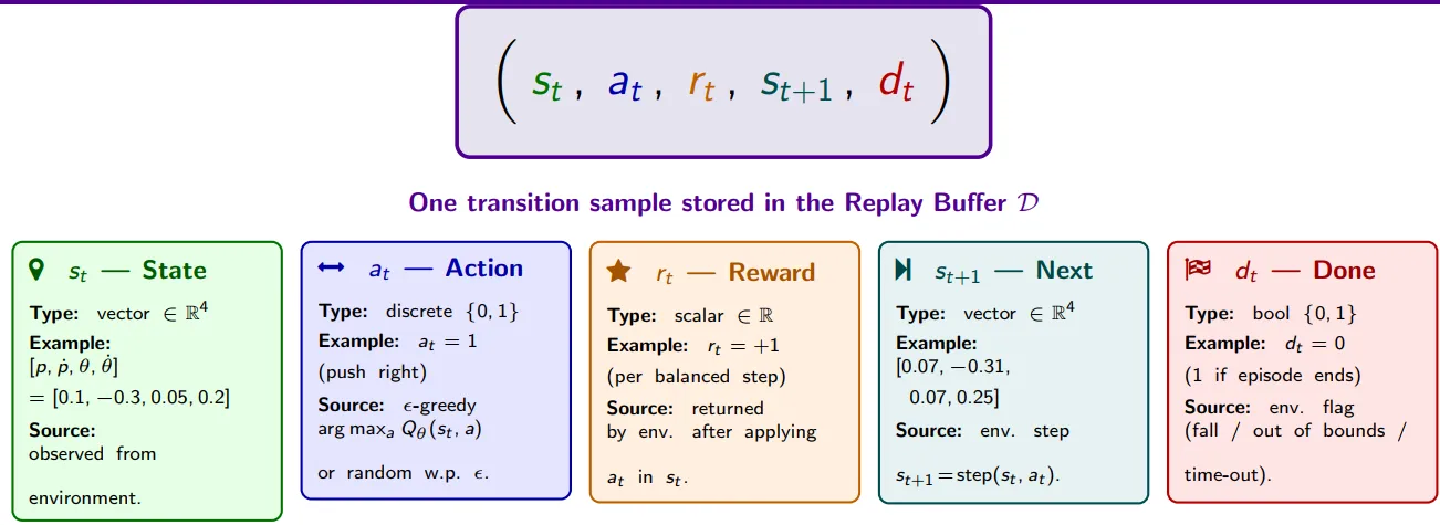
存储经验：将这一步产生的五元组（转移数据 Transition）存入经验回放缓冲区 (Replay Buffer) $\mathcal{D}$ 中：

$$\mathcal{D} \leftarrow \mathcal{D} \cup \big\{ (s_t, a_t, r_t, s_{t+1}, d_t) \big\}$$

更新当前状态：向前推进时间步，将当前状态设为下一状态，进入新的循环：

$$s_t \leftarrow s_{t+1}$$

5-Tuple:

It carries everything needed to evaluate the TD target later: TD Target with Termination

$$y_t = r_t + (1 - d_t) \gamma \max_{a'} Q_{\phi}(s_{t+1}, a')$$

Loss Function

$$\mathcal{L}(\theta) = \big( Q_{\theta}(s_t, a_t) - y_t \big)^2$$

---

Core Training Loop

For every train step：

1. Sampling

从经验回放缓冲区 $\mathcal{D}$ 中随机抽取一个大小为 $B = 128$ 的小批次（Minibatch）数据：

$$\{(s_j, a_j, r_j, s'_j, d_j)\}_{j=1}^B \sim \mathcal{D}$$

2. Target Calculation

Compute Temporal Difference TD using Targe Network目标网络 $Q_\phi$ 计算离策（Off-Policy）的时序差分目标值 $y_j$。此步骤不需要计算梯度：

$$y_j = r_j + \gamma \cdot (1 - d_j) \cdot \max_{a' \in \mathcal{A}} Q_\phi(s'_j, a')$$

3. Loss Calculation

计算目标网络输出的 $y_j$ 与当前网络 $Q_\theta$ 预测值之间的均方误差（MSE）：

$$\mathcal{L}(\theta) = \frac{1}{B} \sum_{j=1}^B \big( y_j - Q_\theta(s_j, a_j) \big)^2$$

4. Gradient Descent

对当前网络参数 $\theta$ 执行梯度下降步以完成参数更新：

$$\theta \leftarrow \theta - \alpha \cdot \nabla_\theta \mathcal{L}(\theta)$$

---

4. Target Network Update

为了保证训练的稳定性，每隔固定的步数（满足 target_frequency 步数要求时），更新目标网络权重 $\phi$：

• Hard Update, $\tau = 1.0$：直接将当前网络的权重完全复制给目标网络： $$\phi \leftarrow \theta$$
• Soft Update, $\tau < 1.0$：让目标网络向当前网络平滑逼近： $$\phi \leftarrow \tau\theta + (1 - \tau)\phi$$

---

Hyper Parameters

Hyper Parameteres	Math	Classical value	Usuage
经验回放区容量	Capacity $N$	10,000	存储历史转移数据 $(s, a, r, s', d)$ 的上限
优化器与学习率	Adam ($\alpha$)	$2.5 \times 10^{-4}$	控制当前网络 $\theta$ 梯度下降的步长
折扣因子	$\gamma$	0.99	衡量未来长远奖励的衰减权重

Weight $\gamma$:

• $\gamma \rightarrow 0$: Greedy, only cares about the immediate reward $r_t$.
• $\gamma \rightarrow \infty$: Strategic, values long term cumulative return.

Moving Target In standard supervised learning, targets(y) are fixed. In RL the target useing the changing network: $\text{Target} \quad y_t = r +\gamma\max_{a'} Q_{\theta}(s',a')$

• When we update weights $\theta$ to approach y_t, the target y_t moves as well.
• Result: Correlation loops, maximization bias, and divergence.

Solution: Twin Network $Q_{\theta}$, a clone of the main network that is frozen in time.

$$y_t = r + \gamma \max_{a'} Q_\phi(s', a')$$

• Main Net$(Q_\theta)$: Updates every step.
• Target Net$(Q_\phi)$: Frozen, Constant.
• Sync: Every C steps, copy weights.

graph LR
    Main --->|Copy slow| Target
    Target --->|target y_t | Main

Practical Design Knobs

1. Exploration Strategy

How do we encourage trying new things?

• $\epsilon$-greedy (Discrete): Flip a coin. With prob $\epsilon$, take random action. Simple.
• Entropy Reg. (Continuous): Add penalty $+\alpha \mathcal{H}(\pi)$ to loss. Keeps policy uncertain to prevent premature convergence.

2. On-Policy vs. Off-Policy

• On-Policy (e.g., PPO): Use data generated only by current $\pi_k$. Stable, but sample inefficient (throws data away).
• Off-Policy (e.g., DDPG, DQN): Use data from any past policy (Replay Buffer). Efficient, but mathematically risky (bias).

3. Stability Hacks (Essential)

Neural Networks hate correlated data. Fixes:

• Replay Buffers: Store $(s, a, r, s')$. Sample random batches to break temporal correlations (i.i.d.).
• Target Networks: Compute loss targets with a frozen network copy. Prevents “chasing your own tail.”

RL Taxonomy / Classifying the Algorithms

1. Action Space

• Discrete: Finite choices (e.g., Left/Right). Output is a probability mass. (Ex: DQN, Q-Learning)
• Continuous: Real-valued vectors (e.g., Torques). Output is a distribution or value. (Ex: DDPG, SAC)

2. Model Usage

• Model-Based: Uses dynamics $f(s, a)$ to plan. High sample efficiency. (Ex: Dyna-Q, AlphaZero)
• Model-Free: Learns mapping $s \rightarrow a$ via trial-and-error. Low bias, easier impl. (Ex: DDPG, DQN)

3. Data Regime (Sampling)

• On-Policy: Learns only from current policy $\pi$. Stable but sample heavy. (Ex: PPO, TRPO)
• Off-Policy: Learns from Replay Buffer (old data). Efficient but complex. (Ex: SAC, DQN)

4. Learning Target (The “Brain”)

• Value-Based: Learns $Q(s, a)$. Implicit policy. (Ex: DQN - Discrete only)
• Policy-Based: Optimizes $\pi_\theta$ directly via gradients. (Ex: REINFORCE)
• Actor-Critic: Hybrid. Actor ($\pi$) acts, Critic ($V$) judges to reduce variance. (Ex: PPO, SAC)

5. Safety & Constraints

• Unconstrained: Maximize $J = \sum r$. Violations punished by negative reward. (Ex: Vanilla RL)
• Constrained (CMDP): Max $J$ s.t. cost $C < d$. Uses Lagrangian multipliers. (Ex: CPO)
• Safe / Filtered: Safety layer (Model/Barrier) overrides dangerous actions. (Ex: MPC-in-loop)